Greetings! In the previous blog post, I applied the Parker-Sochacki method to the Ordinary Differential Equations that make up the motion of a single spring in one dimension. I showed the math implementation on converting the system of First Order Differential Equations into a Maclaurin series for position and Maclaurin series for velocity. I showed code in Matlab and then rendered videos in Houdini.
For this post, we are following the same process applying the Parker-Sochacki method to the motion of a single spring in two dimensions. I will show how I applied the Parker-Sochacki method, code, and then rendered videos from implementing the simulation in Houdini.
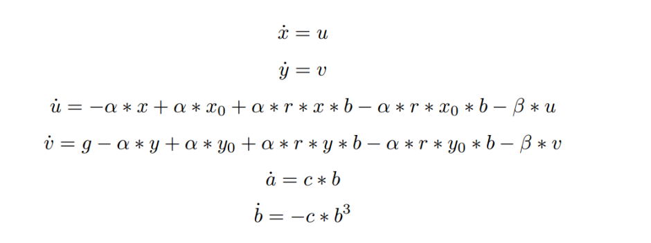
Let’s start by showing the First Order Ordinary Differential equations to update position x, position y, velocity in the x direction u, and velocity in the y direction v:
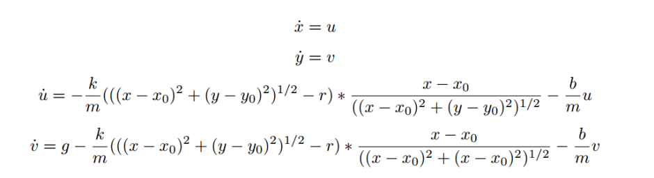
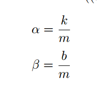
I’ll break this down. k, m, x_0, y_0, b, r, and g are constants. k is the spring constant. m is the mass of the bob. x_0 and y_0 make up the position of the anchor point where the spring is suspended from. b is the damping constant. g is the constant for gravity. r is the rest length. First to make this easier, I will put constant terms together:
To apply the Parker-Sochacki method, I will introduce two auxiliary variables named a and b:
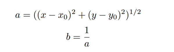
We did this so that it is possible to represent x, y, u, and v as different Maclaurin series. We will also represent a and b as a Maclaurin series:
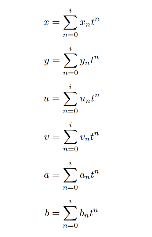
The point of this is to represent x, y, u, v, a, and b all as polynomials that are the Maclaurin series or Taylor series centered at 0. From previous blogs I showed that if we chose to just go to the first term, this becomes a first order method. If we chose to go to the second term setting i to 2, then this becomes a second order method. If we chose to go to the 4th term setting i to 4, this becomes a fourth order method. Generally speaking, increasing the order increases the accuracy of the simulation and often leads to a larger time step than methods like Runge-Kutta 4th order, Verlet, or Forward Euler. For this simulation I chose a 9th order method.
To calculate the nth term, we need to develop a recurrence relationship between the Ordinary Differential Equations. I need to take the derivatives of auxiliary variable a and auxiliary variable b. I will also introduce a variable, c, that I don’t need the derivative of but I need to compute the Maclaurin coefficients: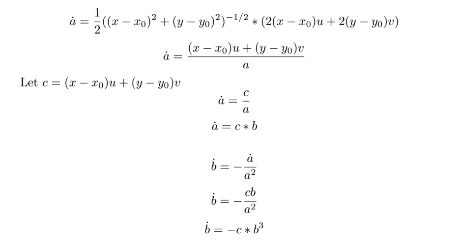
We now have a system of First Order Ordinary Differential Equations. I will put these terms back into velocities u and v so you can see the whole thing together:
To compute the Maclaurin coefficients, I will need to introduce a cauchy product so that I can multiply two power series together. Also, to calculate b, I need to calculate the cube of b. I showed in the 3-body blog that you can take the power of a power series. For this implementation I will calculate the square of b and then use that to calculate the cube of b.
This means I will introduce b2 and b3.
We start with given initial conditions for x, y, u, and v. The initial condition for a is given by the formula for a above and the initial condition for b is given by the formula for b above. It is the reciprocal of a. We then use those initial conditions to create Maclaurin coefficients up to any order we desire. For this simulation, I chose 9th order.
Also, there are constants in the velocities u and v that only need to be computed when i is equal to 1. In the Maclaurin coefficients below, the i+1 for u and v only apply when i is greater than or equal to 1. This recurrence relationship comes from formulas regarding power series.
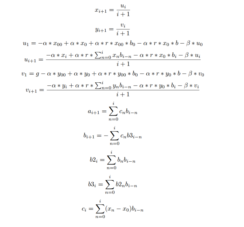
Notice that b2, b3, and c are computing the ith term as opposed to the i+1 term. This is why they do not need a Maclaurin series.
Using this formula, we now can create a Maclaurin series for x, y, u, v, a, and b:

Once the Maclaurin series is computed for every variable, they become the new initial conditions and the process repeats for as many frames as you would like.
I would also like to point out how we put everything together. If you used a numerical method like Forward Euler, Modified Euler, Verlet, or Runge-Kutta 4th order, the section that became auxiliary variable a would have to be recomputed using the square roots in the numerator and denominator with every new frame. Here everything is put together.
Next I will show code in Matlab used to implement this simulation. Because Matlab starts its index at 1, order is set to 10.
% Adam Wermus
% July 9, 2016
% This solves the equations of motion for the 2-D Spring using the
% Parker-Sochacki method
% clear everything
clear all;
clc;
% Parameters
r = 2.5; % rest length
x_0 = 0; % anchor point x
y_0 = 3; % anchor point y
g = -9.81; % gravity
k = 6.0; % spring stiffness
m = 0.5; % mass of bob
damping = 0; % damping constant
alpha = k/m;
beta = damping/m;
% Parker Sochacki setup
order = 10;% order of Maclaurin series
h = 0.04167; % time step
frames = 2500; % number of frames;
% Setup Arrays for Maclaurin coefficients
x = zeros(1, order);
y = zeros(1, order);
u = zeros(1, order);
v = zeros(1, order);
a = zeros(1, order);
b = zeros(1, order);
b2 = zeros(1, order);
b3 = zeros(1, order);
c = zeros(1, order);
% Setup Arrays that store Position and Velocity values
x_sum = zeros(1, frames);
y_sum = zeros(1, frames);
u_sum = zeros(1, frames);
v_sum = zeros(1, frames);
a_sum = zeros(1, frames);
b_sum = zeros(1, frames);
% Initial Conditions
x(1) = 0;
y(1) = -0.31667;
u(1) = 1.5;
v(1) = 1.7;
a(1) = ((x(1) – x_0).^2 + (y(1) – y_0).^2).^(1./2);
b(1) = 1./a(1);
% Initial arrays
x_sum(1) = x(1);
y_sum(1) = y(1);
u_sum(1) = u(1);
v_sum(1) = v(1);
a_sum(1) = a(1);
b_sum(1) = b(1);
% Iterate through every frame
for j = 2:frames
% 1st
c(1) = ((x(1) – x_0).*u(1)) + (y(1) – y_0).*v(1);
b2(1) = b(1).*b(1);
b3(1) = b2(1).*b(1);
% Second setup
x(2) = u(1);
y(2) = v(1);
u(2) = -alpha.*x(1) + alpha.*x_0 + alpha.*r.*x(1).*b(1) – alpha.*r.*x_0.*b(1) – beta.*u(1);
v(2) = g – alpha.*y(1) + alpha.*y_0 + alpha.*r.*y(1).*b(1) – alpha.*r.*y_0*b(1) – beta.*v(1);
a(2) = c(1).*b(1);
b(2) = -c(1).*b3(1);
% Maclaurin coefficients
for i = 2:order-1
% cauchy product for b2
cp_b2 = 0;
for k = 1:i
cp_b2 = cp_b2 + (b(k).*b(i+1-k));
end
b2(i) = cp_b2;
% cauchy product for b3
cp_b3 = 0;
for k = 1:i
cp_b3 = cp_b3 + (b2(k).*b(i+1-k));
end
b3(i) = cp_b3;
% cauchy product for c
cp_c = 0;
for k = 1:i
cp_c = cp_c + ((x(k)-x_0).*u(i+1-k));
cp_c = cp_c + ((y(k)-y_0).*v(i+1-k));
end
c(i) = cp_c;
% Update x and y position
x(i+1) = u(i) / i;
y(i+1) = v(i) / i;
% Velocity update
cp_u = 0;
cp_v = 0;
for k = 1:i
cp_u = cp_u + (x(k).*b(i+1-k));
cp_v = cp_v + (y(k).*b(i+1-k));
end
cp_u = alpha.*r.*cp_u;
cp_v = alpha.*r.*cp_v;
cp_u = cp_u – (alpha.*x(i));
cp_v = cp_v – (alpha.*y(i));
cp_u = cp_u – (alpha.*r.*x_0.*b(i));
cp_v = cp_v – (alpha.*r.*y_0.*b(i));
cp_u = cp_u – (beta.*u(i));
cp_v = cp_v – (beta.*v(i));
u(i+1) = cp_u / i;
v(i+1) = cp_v / i;
% cauchy product for a and b
cp_a = 0;
cp_b = 0;
for k = 1:i
cp_a = cp_a + (c(k).*b(i+1-k));
cp_b = cp_b + (c(k).*b3(i+1-k));
end
a(i+1) = cp_a / i;
b(i+1) = -cp_b / i;
end
% Temporary sums
x_sum_temp = 0;
y_sum_temp = 0;
u_sum_temp = 0;
v_sum_temp = 0;
a_sum_temp = 0;
b_sum_temp = 0;
% Compute Maclaurin series
for i = 1:order-1
x_sum_temp = x_sum_temp + (x(i)*h^(i-1));
y_sum_temp = y_sum_temp + (y(i)*h^(i-1));
u_sum_temp = u_sum_temp + (u(i)*h^(i-1));
v_sum_temp = v_sum_temp + (v(i)*h^(i-1));
a_sum_temp = a_sum_temp + (a(i)*h^(i-1));
b_sum_temp = b_sum_temp + (b(i)*h^(i-1));
end
% Store Maclaurin series into sum array
x_sum(j) = x_sum_temp;
y_sum(j) = y_sum_temp;
u_sum(j) = u_sum_temp;
v_sum(j) = v_sum_temp;
a_sum(j) = a_sum_temp;
b_sum(j) = b_sum_temp;
% Reset initial conditions
x(1) = x_sum(j);
y(1) = y_sum(j);
u(1) = u_sum(j);
v(1) = v_sum(j);
a(1) = a_sum(j);
b(1) = b_sum(j);
end
% Plot Results
plot(x_sum,y_sum, ‘k-‘);
title(‘Parker-Sochacki Single Spring 2D’)
xlabel(‘x position’);
ylabel(‘y position’);
legend(‘Motion of a 2D Bob’);
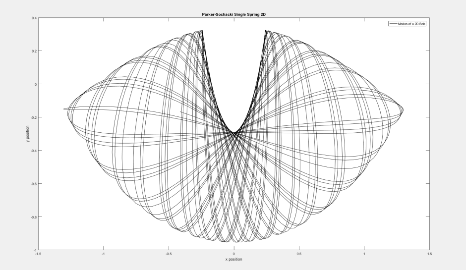
Damping is set to 0 making a beautiful picture of the bob moving back and forth. It does not go to rest.
This simulation was also implemented in Houdini. In this first video, the time step is set to 1/12 and the order of the Maclaurin series is set to 9. Damping is set to zero so that the bob does not go to rest. The Parker-Sochacki implementation is in the sphere. I then used a wiresolver and static solver to constrain the coil.
For this next video, I set the damping to 0.2 so that the bob will stop moving around. I also gave it a higher initial velocity in the x direction so it begins to move to the right before constraints pull it in.
Thank you for taking the time to go through this! I hope this gives a better understanding of using the Parker-Sochacki method.
