In the last blog, I showed that Parker-Sochacki demonstrates properties of conserving energy on the Simple Pendulum model. I have since implemented the following numerical methods to solve the equations of motion for the Simple Pendulum: Forward Euler, Semi-Implicit Euler, Velocity Verlet, Runge-Kutta 2 Midpoint Method, and Runge-Kutta 4th Order. They will be compared to Parker-Sochacki. This blog shows results of how the total energy is handled under the same initial conditions for all of these methods when the angular displacement, theta, looks as follows:

Aside from Forward Euler, all of the other methods could handle a time step of 1/30 and have this up and down sine like motion for their theta update before I tested their total energy. I will show plots of Forward Euler, Semi-Implicit Euler, Velocity Verlet, Runge-Kutta 2 Midpoint, and Runge-Kutta 4. Then I will show 3 plots of Parker-Sochacki at different orders.
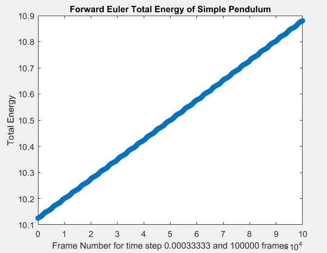
Forward Euler gains energy. Look at how small the time step is to make this work and it is still steadily gaining energy as the simulation goes on.
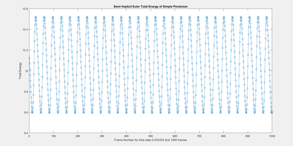
Semi-Implicit Euler is a symplectic integrator so this result is expected. The total energy appears stable for the entire simulation. The value range is from around 9.6 to a little above 10.5.
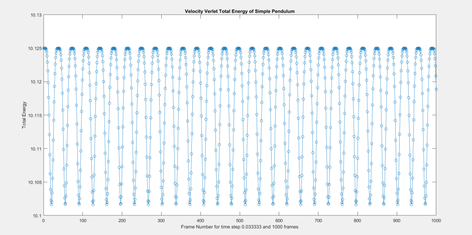
Velocity Verlet is also a symplectic integrator. This does a better job than Semi-Implicit Euler at conserving energy. The lowest value is around 10.101 to 10.125.
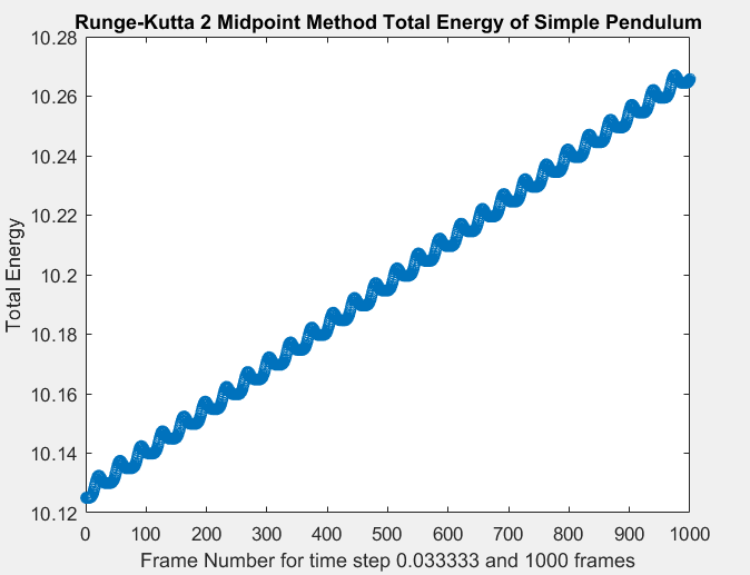
Runge-Kutta 2 Midpoint Method is a second order explicit method that gains energy from a little over 10.12 to a little over 10.26. This gains energy at a slower rate than Forward Euler.
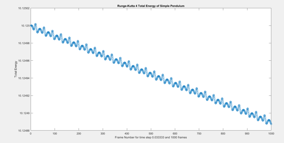
Runge-Kutta 4th Order is losing energy but for the entire simulation it lowered from around 10.125 to 10.12488. It is losing energy but the range is smaller than Velocity Verlet. If this simulation went longer, it would lose more energy.
Now we will look at 3 Parker-Sochacki plots under different orders: 4, 5, and 20:
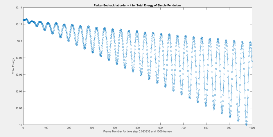
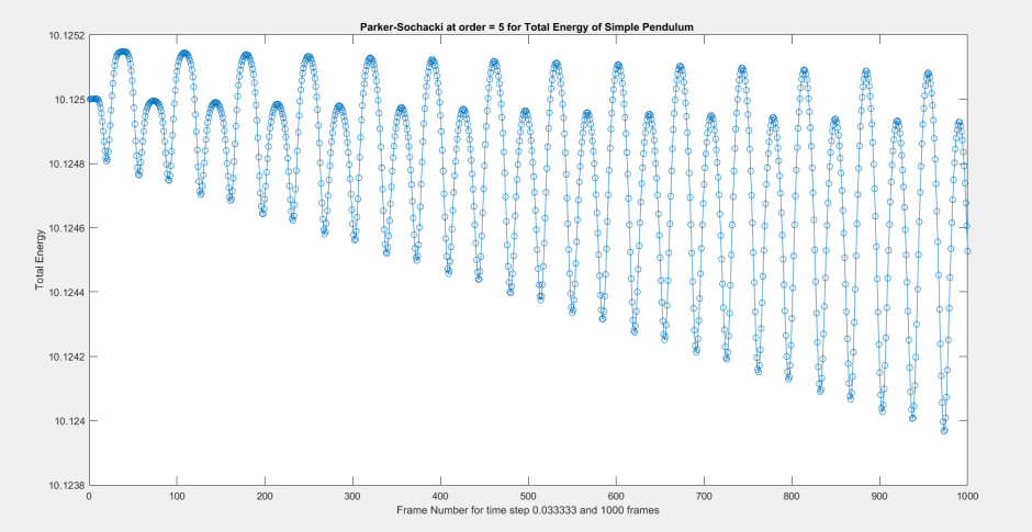
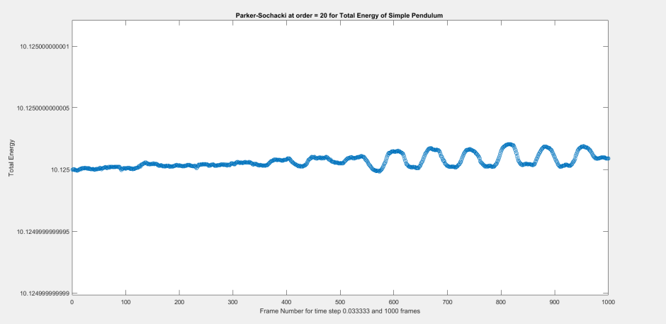
The first plot shows that Parker-Sochacki Order 4 is similar but not the same as Runge-Kutta 4. Parker-Sochacki Order 5 also loses energy but performs better than Parker-Sochacki Order 4. Look at Parker-Sochacki Order 20-Look at how many decimal places the window goes to. The total energy is around 10.125 but the bar above it is 10.1250000000005 and the bar below it is 10.1249999999995. The other methods do not come close to that.
This shows for this physical simulation that Parker-Sochacki at a higher order does a better job at conserving energy than the other methods it was compared to: Forward Euler, Semi-Implicit Euler, Velocity Verlet, Runge-Kutta 2 Midpoint Method, and Runge-Kutta 4th Order.
