Greetings!
I applied the Parker-Sochacki method to Ordinary Differential Equations that describe the 2D motion of a projectile with gravity and drag forces. The drag force makes it an Ordinary Differential Equation that has no analytical solution. Applying Parker-Sochacki makes it possible to update the position and velocity of the projectiles as a Maclaurin series up to any order desired.
Applying Parker-Sochacki led to larger time steps than Runge-Kutta 4th Order. Those larger time steps may not be needed for this specific problem but there is a lot of potential here for other projectile problems. This could expand to Buoyancy forces, Coriolis forces, or other forces in animation.
I also want to note that Dr. Rudmin from James Madison University published a paper that covers this problem. The only difference is that he set constants to 1 and I wanted to keep true values for those constants.
I show two renders, talk about the implementation, show code, images with and without drag, and show that a higher order eliminates an error.
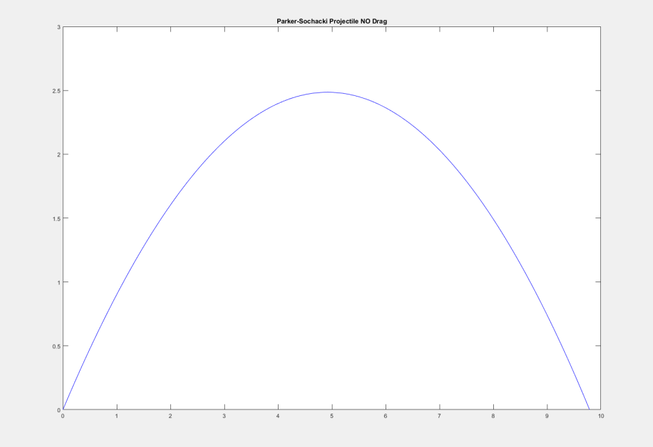
We’ll start with what to look at. There are two videos below. The first is a soccer ball that I modeled traveling through the air without drag. It was given an initial position and velocity and has only gravity acting on it. The motion “appears” like a parabola:
Projectile without Drag:
Drag was set to 0. For this next video, Drag was turned on. Notice how the motion looks like a skewed parabola.
Projectile with Drag:
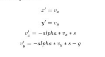
Now is the math section. We start with four First Order Ordinary Differential Equations: 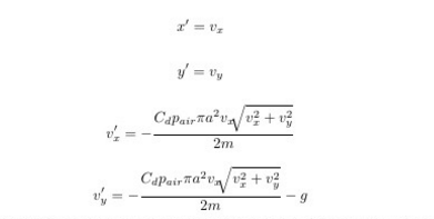
x’ is the x velocity
y’ is the y velocity
v_x’ is the x acceleration
v_y’ is the y acceleration
where C_d is the drag coefficient
p_air is the density of the air
pi is 3.14159
a is the radius of the soccer ball
m is the mass of the ball
These are all constants that are combined and called alpha.
alpha = (C_d * p_air * pi * a^2) / 2m
Gravity is only used in v_y’
Also, I used the same values that were in the Brigham Young University Physics manual. If you google BYU Physics 330, this should be available:
https://www.physics.byu.edu/Courses/Computational/phys330.aspx
Here are the values:
C_d = 0.35
a = 0.037
g = 9.81
p_air = 1.2
m = 0.145
For Houdini, they were given initial conditions:
x(0) = 0; y(0) = 0
v_x(0) = 10; v_y(0) = 0
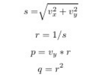
Here is the Parker-Sochacki part: putting one variable into the square root of v_x^2 + v_y^2. We call it s so that it now looks like this:
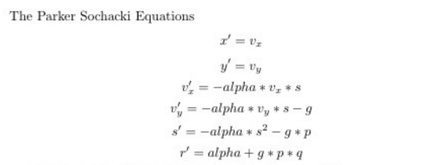
For this to be Parker-Sochacki, we need to take the derivative of s. This is an ODE that comes back beautifully(it uses chain rule)
alpha and g are constants. s^2 is a cauchy product and p is an auxiliary variable I will show in a moment. I am not multiplying by more than 2 variables at once. This is in a form that depends on itself and uses only multiplication and subtraction. Here are all of the auxiliary variables together:
So all of the ODEs that are needed(ignore p and q for a moment)
What you can get from this is we went from 4 ODEs to 6 with 2 extra variables p and q.
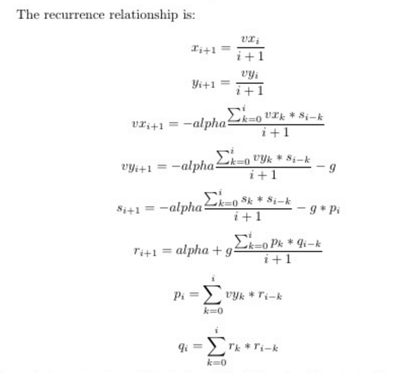
Using power series formulas, we now have the following recurrence relationship needed to turn x, y, vx, and vy into a Maclaurin series up to any order. The i is the coefficient for the Maclaurin series.
This setup is what makes it possible to update the position x and y in a Maclaurin Series.
Next I will show code in Matlab and we will play with the time step. This code implements a low almost non existent drag:
————————————————————————————————————————————————————
% Adam Wermus
% June 8, 2015
% This program solves the following ODEs
% dx/dt = v_x
% dv_x/dt = -(C_d*rho_air*pi*a^2*v_x*sqrt(v_x^2+v_y^2)) / 2m
% dy/dt = v_y
% dv_y/dt = -((C_d*rho_air*pi*a^2*v_y*sqrt(v_x^2+v_y^2)) / 2m) – g
% The Parker Sochacki Equations
% dx/dt = v_x
% dy/dt = v_y
% dv_x/dt = -alpha*v_x*s
% dv_y/dt = -alpha*v_y*s – g
% ds/dt = -alpha*s^2 – g*p
% dr/dt = alpha + g*p*q
% HERE ARE THE AUXILIARY VARIABLES
% s = sqrt(v_x^2 + v_y^2)
% r = 1/s
% p = v_y*r
% q = r^2
% Clear everything
clc;
clear all;
close all;
% Constants
Cd = 0.35; % drag coefficient
a = 0.037; % radius of the ball in meters
g = 9.81; % gravity
rho_air = 1.2; % density of the air
m = 0.145; % mass of the ball
% Combine constants into one
alpha = (Cd*rho_air*pi*a.^2)./(2*m);
% Declare variables for Parker-Sochacki Implementation
order = 20; % order for power series
t = 0.01; % time step
frames = 500; % number of iterations
% initial conditions for position
x(1) = 0;
y(1) = 0;
% initial conditions for velocity
v_not = 10; % meters/sec
vx(1) = v_not.*cosd(45); % converts degrees to radians
vy(1) = v_not.*sind(45);
% Initial conditions for auxiliary variables
s(1) = sqrt(vx(1)^2 + vy(1)^2);
r(1) = 1./s(1);
p(1) = vy(1)*r(1);
q(1) = r(1)*r(1);
% Declare These are the power series sums
x_sum = zeros(1,frames);
y_sum = zeros(1,frames);
vx_sum = zeros(1,frames);
vy_sum = zeros(1, frames);
s_sum = zeros(1, frames);
r_sum = zeros(1, frames);
p_sum = zeros(1, frames);
q_sum = zeros(1, frames);
% Give initial value sums
x_sum(1) = x(1);
y_sum(1) = y(1);
vx_sum(1) = vx(1);
vy_sum(1) = vy(1);
s_sum(1) = s(1);
r_sum(1) = r(1);
p_sum(1) = p(1);
q_sum(1) = q(1);
% This for loop updates the frames
for iterate = 2:frames
% Setup cauchy product
cp_vx = 0;
cp_vy = 0;
cp_s = 0;
cp_r = 0;
cp_p = 0;
cp_q = 0;
% Calculate second term where needed
x(2) = vx(1);
y(2) = vy(1);
vx(2) = -alpha*vx(1)*s(1);
vy(2) = -alpha*vy(1)*s(1) – g;
s(2) = -alpha*s(1)*s(1) – g*p(1);
r(2) = alpha + g*p(1)*q(1);
p(2) = vy(1)*r(1);
q(2) = r(1)*r(1);
% Calculate Coefficients
for i = 2 : order-1
% Setup cauchy product
cp_vx = 0;
cp_vy = 0;
cp_s = 0;
cp_r = 0;
cp_p = 0;
cp_q = 0;
% Position
x(i+1) = vx(i)/i;
y(i+1) = vy(i)/i;
% Cauchy Products
% Compute Cauchy Products
for k =1:i
cp_vx = cp_vx + ((vx(k)*s(i+1-k))/i);
cp_vy = cp_vy + ((vy(k)*s(i+1-k))/i);
cp_s = cp_s + ((s(k)*s(i+1-k) + g*p(i))/i);
cp_r = cp_r + ((p(k)*q(i+1-k))/i);
cp_p = cp_p + ((vy(k)*r(i+1-k))/i);
cp_q = cp_q + ((r(k)*r(i+1-k))/i);
end
% Put in cauchy product to coefficient
vx(i+1) = -alpha*cp_vx; % vx
vy(i+1) = -alpha*cp_vy; % vy
s(i+1) = -alpha*cp_s; % s
r(i+1) = g*cp_r; % r
p(i+1) = cp_p; % p
q(i+1) = cp_q; % q
end
% Setup sums
x_temp_sum = 0;
y_temp_sum = 0;
vx_temp_sum = 0;
vy_temp_sum = 0;
s_temp_sum = 0;
r_temp_sum = 0;
p_temp_sum = 0;
q_temp_sum = 0;
% Compute Power series
for i = 1:order
x_temp_sum = x_temp_sum + (x(i)*t^(i-1));
y_temp_sum = y_temp_sum + (y(i)*t^(i-1));
vx_temp_sum = vx_temp_sum + (vx(i)*t^(i-1));
vy_temp_sum = vy_temp_sum + (vy(i)*t^(i-1));
s_temp_sum = s_temp_sum + (s(i)*t^(i-1));
r_temp_sum = r_temp_sum + (r(i)*t^(i-1));
p_temp_sum = p_temp_sum + (p(i)*t^(i-1));
q_temp_sum = q_temp_sum + (q(i)*t^(i-1));
end
% Put in power series to store in array
x_sum(iterate) = x_temp_sum;
y_sum(iterate) = y_temp_sum;
vx_sum(iterate) = vx_temp_sum;
vy_sum(iterate) = vy_temp_sum;
s_sum(iterate) = s_temp_sum;
r_sum(iterate) = r_temp_sum;
p_sum(iterate) = p_temp_sum;
q_sum(iterate) = q_temp_sum;
% reset initial conditions
x(1) = x_temp_sum;
y(1) = y_temp_sum;
vx(1) = vx_temp_sum;
vy(1) = vy_temp_sum;
s(1) = s_temp_sum;
r(1) = r_temp_sum;
p(1) = p_temp_sum;
q(1) = q_temp_sum;
end
% Plot exact solution
plot(x_sum,y_sum, ‘b’);
title(‘Parker-Sochacki Projectile NO Drag’);
ylim([0, 3]); % stop the plot when you get to zero
————————————————————————————————————————————————————
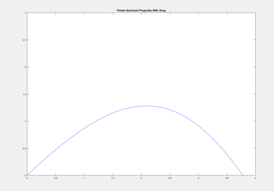
Now this next image I multiplied alpha by 50:
You can see the motion is skewed and it does not go nearly as high.
Now we will compare this with Runge-Kutta 4th Order.
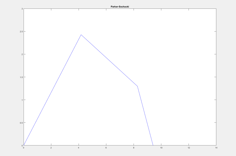
Next we have an image where the time step is much larger: 0.6
This image has the same projectile at order 5 in Matlab(about the same accuracy as Runge-Kutta 4th Order). 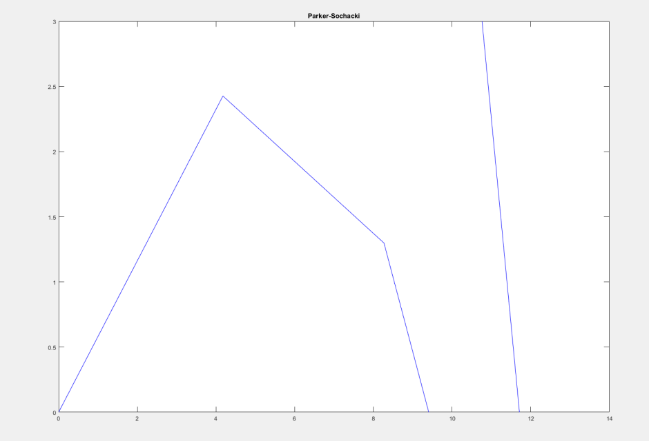
It is messed up. The projectile goes up and down but then has some funky pattern near 12. Look what happens when I increase the order by 1 to 6:
The error is gone. Parker-Sochacki, while these are huge steps, is able to take larger time steps and still maintain its accuracy. This is something that lower order numerical methods cannot achieve.
This is the whole point: Parker-Sochacki’s accuracy is higher and can take larger time steps. I used order 6 in Matlab. The higher the order, the more expensive the computation.
