There are previous blog posts I have written about applying the Parker-Sochacki method to the 2 and 3-body gravity problems. I discussed results(showing benefits of a higher order method and how Parker-Sochacki does well against close encounters(bodies that are very close).
This blog picks up from the previous blogs. I still take the power of a power series so I skip auxiliary variable s2.
At long last, I have generalized the 3-body problem into an N-body problem. The code posted below can be modified to as many bodies as you want. All you need to do is change num_of_bodies to the number of bodies in your simulation, add, remove, or change the initial conditions, and then adjust how you plot the final solution.
First, I will show the Ordinary Differential Equations again from a previous post, then I will show the code, then I will discuss what I did involving matrices, then I will show output for number of bodies set to 2, 3, and 5.
In 3D, these are the equations of motion to update the position and velocity of particle j:
I implemented the n-body problem in 2D. There is a previous blog where I implemented a 3D version of the 2-body problem in Houdini.
For the 3-body problem, I had an auxiliary variable represent particle 1 to particle 2, particle 1 to particle 3, and particle 2 to particle 3. It was tedious being hard coded. I used matrices in Matlab to generalize this.
I use the same notation that is done in the published Parker-Sochacki n-body papers out of respect. They were the geniuses to create this. The main difference between my implementation is that I skip auxiliary variable s2.
Matlab Code for number of bodies set to 5:
% Adam Wermus
% July 1, 2016
% This program uses the Parker-Sochacki Method to solve the n-Body problem
% in 2 dimensions
% clear everything
close all;
clear all;
clc;
% Parameters
% num_of_bodies is the number of bodies
% G is the gravitational constant.
% Next are the masses for every “body”
num_of_bodies = 5;
G = 1;
m(1) = 1;
m(2) = 1;
m(3) = 1;
m(4) = 1;
m(5) = 1.5;
% Declare variables for Parker-Sochacki Implementation
order = 7; % order of Maclaurin series
t = 0.005; % time step
frames = 180; % number of iterations
power = 3; % power of a power series taking s to s^3
% Create arrays for all Maclaurin coefficients for position and velocity in
% the x and y directions
x_pos = zeros(num_of_bodies, order-1);
y_pos = zeros(num_of_bodies, order-1);
vx = zeros(num_of_bodies, order-1);
vy = zeros(num_of_bodies, order-1);
% Create arrays for the auxiliary variables s, s3, and a
s = zeros(num_of_bodies,num_of_bodies,order-1);
s3 = zeros(num_of_bodies,num_of_bodies,order-1);
a = zeros(num_of_bodies,num_of_bodies,order-1);
% initial mass 1 conditions
x_pos(1,1) = 0.55;
vx(1,1) = 0;
y_pos(1,1) = 0.27;
vy(1,1) = 0.23;
% initial mass 2 conditions
x_pos(2,1) = 0.30;
vx(2,1) = 0;
y_pos(2,1) = 0.27;
vy(2,1) = -2.42;
% initial mass 3 conditions
x_pos(3,1) = -0.30;
vx(3,1) = 0;
y_pos(3,1) = 0.27;
vy(3,1) = 2.42;
% initial mass 4 conditions
x_pos(4,1) = -0.55;
vx(4,1) = 0;
y_pos(4,1) = 0.27;
vy(4,1) = -0.23;
% initial mass 5 conditions
x_pos(5,1) = 0.0;
vx(5,1) = 0;
y_pos(5,1) = -0.72;
vy(5,1) = 0;
% initialize x position, y position, velocity x, velocity y for the bodies
x_pos_sum = zeros(num_of_bodies,frames);
y_pos_sum = zeros(num_of_bodies,frames);
vx_sum = zeros(num_of_bodies, frames);
vy_sum = zeros(num_of_bodies, frames);
% This loop gives the first frame values of position and velocity to the
% arrays
for n = 1:num_of_bodies
x_pos_sum(n,1) = x_pos(n,1);
y_pos_sum(n,1) = y_pos(n,1);
vx_sum(n,1) = vx(n,1);
vy_sum(n,1) = vy(n,1);
end
% This for loop updates the frames
for j = 2:frames
% Calculate Coefficients
for iterate = 1 : order-1
% initialize auxiliary variables
% This for loop guarantees that we won’t go to the same “body”
% This loop does half of the matrix calculation because it is
% symmetric(the distance between point 1 and point 2 is the same as
% the distance between point 2 and point 1
% We fill in the other parts in the next loop
for n = 1:num_of_bodies
for p = n+1:num_of_bodies
s(n,p,1) = 1./sqrt((x_pos(n,1) – x_pos(p,1)).^2 + (y_pos(n,1) – y_pos(p,1)).^2);
end
end
% This avoids doing multiple calculations over again. This is a
% symmetric matrix with diagonal zeros(actually the diagonals for
% this are infinity
for n = 1:num_of_bodies
for p = n+1:num_of_bodies
s(p,n,1) = s(n,p,1);
end
end
% Cauchy Product Arrays
cp_vx = zeros(num_of_bodies);
cp_vy = zeros(num_of_bodies);
cp_a = zeros(num_of_bodies, num_of_bodies);
cp_s = zeros(num_of_bodies, num_of_bodies); % cauchy product matrix for auxiliary variable s
cp_s3 = zeros(num_of_bodies, num_of_bodies); % cauchy product matrix for auxiliary variable s3
% Cauchy Products s3, v3, x3 first setup
if iterate == 1
% Computes initial condition of first half of matrix
for n = 1:num_of_bodies
for p = n+1:num_of_bodies
s3(n,p,1) = s(n,p,1) * s(n,p,1) * s(n,p,1);
end
end
% Fills in second half of matrix
for n = 1:num_of_bodies
for p = n+1:num_of_bodies
s3(p,n,1) = s3(n,p,1);
end
end
% For all other non-initial auxiliary variable coefficients
else
for k = 2:iterate
% Putting quick here avoids calculating this muliple times
quick = 1/(iterate – 1);
% Here we sum through the bodies to get our s3 term. This
% uses a power of a power series. We only do half of the
% matrix because it is symmetric. The other half is filled
% out later
for n = 1:num_of_bodies
for p = n+1:num_of_bodies
cp_s3(n,p) = cp_s3(n,p) + ((k-1) * power – (iterate – 1) + (k-1)) * (s(n, p, k) * s3(n, p, iterate + 1 – k));
end
end
end
% This part comes from the last chunk of the formula to take a
% power of a power series
for n = 1:num_of_bodies
for p = n+1:num_of_bodies
cp_s3(n,p) = cp_s3(n,p) * (quick / s(n,p,1)) ;
end
end
end
% The formula only applies to the non-initial condition
if iterate >= 2
for n = 1:num_of_bodies
for p = n+1:num_of_bodies
s3(n,p,iterate) = cp_s3(n,p);
end
end
% Fill in second half of s3 matrix
for n = 1:num_of_bodies
for p = n+1:num_of_bodies
s3(p,n,iterate) = s3(n,p,iterate);
end
end
end
% Cauchy Product for auxiliary variable a
% We cover only half of the matrix because it is symmetric
for k = 1:iterate
for n = 1:num_of_bodies
for p = n+1:num_of_bodies
cp_a(n,p) = cp_a(n,p) + ((x_pos(n,k) – x_pos(p,k)).*(vx(n,(iterate+1)-k)-vx(p,(iterate+1)-k)) + (y_pos(n,k) – y_pos(p,k)).*(vy(n,(iterate+1)-k)-vy(p,(iterate+1)-k)));
end
end
end
% Fills in second half of matrix
for n = 1:num_of_bodies
for p = n+1:num_of_bodies
cp_a(p,n) = cp_a(n,p);
end
end
% Fill in values into auxiliary variable a from cauchy product
% calculation above
for n = 1:num_of_bodies
for p = 1:num_of_bodies
a(n,p,iterate) = cp_a(n,p);
end
end
% Cauchy Product for auxiliary variable s
% We cover only half of the matrix because it is symmetric
for k = 1:iterate
for n = 1:num_of_bodies
for p = n+1:num_of_bodies
cp_s(n,p) = cp_s(n,p) + (s3(n,p,k)*a(n,p,(iterate+1)-k));
end
end
end
% Fills in second half of matrix s
for n = 1:num_of_bodies
for p = n+1:num_of_bodies
cp_s(p,n) = cp_s(n,p);
end
end
% Fill in values into auxiliary variable a from cauchy product
% calculation above
for n = 1:num_of_bodies
for p = 1:num_of_bodies
s(n,p,iterate + 1) = -cp_s(n,p)/iterate;
end
end
% Updates position for all bodies
for n = 1 : num_of_bodies
x_pos(n,iterate+1) = vx(n,iterate)/iterate;
y_pos(n,iterate+1) = vy(n,iterate)/iterate;
end
% Cauchy Products for Velocity
for k = 1:iterate
% We need to sum over all of the neighboring bodies. This is
% the Cauchy Product of the velocity
for n = 1:num_of_bodies
for p = 1:num_of_bodies
cp_vx(n) = cp_vx(n) + (G*m(p)*(x_pos(p,k)-x_pos(n,k))*s3(n,p,(iterate+1)-k));
cp_vy(n) = cp_vy(n) + (G*m(p)*(y_pos(p,k)-y_pos(n,k))*s3(n,p,(iterate+1)-k));
end
end
end
% We will now put the values from the caucy product into the
% velocity array
for n = 1 : num_of_bodies
vx(n,iterate+1) = cp_vx(n)/iterate;
vy(n,iterate+1) = cp_vy(n)/iterate;
end
end
% Setup sums for the bodies
x_temp_sum = zeros(num_of_bodies);
y_temp_sum = zeros(num_of_bodies);
vx_temp_sum = zeros(num_of_bodies);
vy_temp_sum = zeros(num_of_bodies);
% Compute Power series
for i = 1:order-1
for n = 1:num_of_bodies
x_temp_sum(n) = x_temp_sum(n) + (x_pos(n,i)*t^(i-1));
y_temp_sum(n) = y_temp_sum(n) + (y_pos(n,i)*t^(i-1));
vx_temp_sum(n) = vx_temp_sum(n) + (vx(n,i)*t^(i-1));
vy_temp_sum(n) = vy_temp_sum(n) + (vy(n,i)*t^(i-1));
end
end
% Put in power series to store in array
for n = 1:num_of_bodies
x_pos_sum(n,j) = x_temp_sum(n);
y_pos_sum(n,j) = y_temp_sum(n);
vx_sum(n,j) = vx_temp_sum(n);
vy_sum(n,j) = vy_temp_sum(n);
end
% Reset Initial Conditions
for n = 1:num_of_bodies
x_pos(n,1) = x_temp_sum(n);
y_pos(n,1) = y_temp_sum(n);
vx(n,1) = vx_temp_sum(n);
vy(n,1) = vy_temp_sum(n);
end
end
% Plot Results
% We know this is a 3-body version of n-body. This has to change as the
% number of bodies change.
% This creates 1-D Arrays for x and y of every “body”
x1 = x_pos_sum(1,:);
y1 = y_pos_sum(1,:);
x2 = x_pos_sum(2,:);
y2 = y_pos_sum(2,:);
x3 = x_pos_sum(3,:);
y3 = y_pos_sum(3,:);
x4 = x_pos_sum(4,:);
y4 = y_pos_sum(4,:);
x5 = x_pos_sum(5,:);
y5 = y_pos_sum(5,:);
% Plot results
plot(x1,y1,’c-‘, x2,y2, ‘k’, x3,y3,’r’, x4,y4, ‘b’, x5,y5,’g.’);
legend(‘mass 1’, ‘mass 2’, ‘mass 3’, ‘mass 4’, ‘mass 5’);
title(‘Parker-Sochacki N-Body Implementation where N = 5’);
Here is how this is broken down:
I have an x position matrix n by k where n is the particle and k is the order.
I have a y position matrix n by k where n is the particle and k is the order.
I have an x velocity matrix n by k where n is the particle and k is the order.
I have a y velocity matrix n by k where n is the particle and k is the order.
I have an auxiliary variable matrix for s,s3,and a that is n by n by k. This distinguishes the relationship between particles for order k.
I have matrices that are used to calculate the cauchy products for velocity, s, s3, and a. These matrices are n by n.
In the code, there are a lot of spots where I sum over all neighboring particles.
Here is an important note about the matrices for s, s3, and a. The relationship between particle 1 and particle 2 is the same as the relationship between particle 2 and particle 1. All 3 of these matrices are symmetric. I only need to compute half of those values(you can see this in the code where I fill half of one matrix and use that to fill in the other half). The diagonals for s, s3, and a were set to zero. The diagonals for s should be infinity because I would be dividing by zero.
Regarding s3, I still took the power of a power series as opposed to using cauchy products to compute s2, and then using cauchy products to compute s3. In a previous blog, I found that taking a power of a power series is faster. In all of the n-body Parker-Sochacki papers I have come across, I have not seen this type of implementation where s2 is skipped. I am not sure why.
When I implemented the 3-body replica in a previous blog, the simulation time took around 5 seconds as opposed to 1. The way I generalized this algorithm led to a greater computation cost.
Next I will show outputs for different initial conditions that I found online. I will show the image followed by the initial conditions in case you would be interested in trying this yourself.
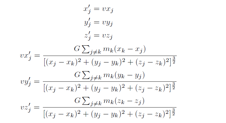
This is the original 2-body problem that I showed a few months ago.
number of bodies = 2
G = 1
mass of particle 1 = 1
mass of particle 2 = 2
Order of Maclaurin series = 22
time step = 0.04167
number of frames = 10000
x_particle 1 = 1
velocity_x_particle 1 = 0.65
y_particle 1 = 0.5
velocity_y_particle 1 = 0.2
x_particle 2 = -1
velocity_x_particle 2 = -0.45
y_particle 2 = -0.3
velocity_y_particle 2 = 0.3
This is the original 3-body problem that I showed a few months ago.
number of bodies = 3
G = 1
mass of particle 1 = 0.6
mass of particle 2 = 0.1001
mass of particle 3 = 0.00101
Order of Maclaurin series = 30
time step = 0.001
number of frames = 2125
x_particle 1 = 0
velocity_x_particle 1 = 0.6
y_particle 1 = 1.95
velocity_y_particle 1 = 0.5
x_particle 2 = 0
velocity_x_particle 2 = 2.828
y_particle 2 = 2
velocity_y_particle 2 = 0
x_particle 3 = 0
velocity_x_particle 3 = 0
y_particle 3 = 2.1
velocity_y_particle 3 = 0

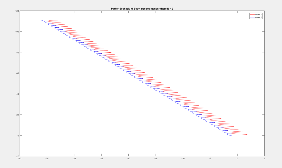
3-Body Problem where the red particle that cannot be seen is the center of mass. The blue and black particles are going around it
number of bodies = 3
G = 1
mass of particle 1 = 1
mass of particle 2 = 1
mass of particle 3 = 2
Order of Maclaurin series = 30
time step = 0.1
number of frames = 2000
x_particle 1 = -1
velocity_x_particle 1 = 0
y_particle 1 = 0
velocity_y_particle 1 = 1
x_particle 2 = 1
velocity_x_particle 2 = 0
y_particle 2 = 0
velocity_y_particle 2 = -1
x_particle 3 = 0
velocity_x_particle 3 = 0
y_particle 3 = 0
velocity_y_particle 3 = 0
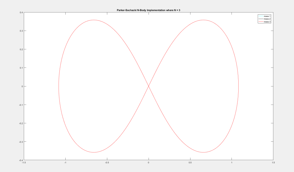
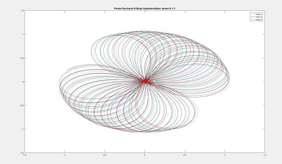
This is the 3-body problem that simulates a figure 8. All 3 bodies are tracing the same path, which is why you only see one particle.
number of bodies = 3
G = 1
mass of particle 1 = 1
mass of particle 2 = 1
mass of particle 3 = 1
Order of Maclaurin series = 10
time step = 0.001
number of frames = 9000
x_particle 1 = 0.97000436
velocity_x_particle 1 = 0.466203685
y_particle 1 = -0.24308753
velocity_y_particle 1 = 0.43236573
x_particle 2 = -0.97000436
velocity_x_particle 2 = 0.466203685
y_particle 2 = 0.24308753
velocity_y_particle 2 = 0.43236573
x_particle 3 = 0
velocity_x_particle 3 = -0.93240737
y_particle 3 = 0
velocity_y_particle 3 = -0.86473146
This is a 3-body problem where I only modified the x position of particle 1 from the above simulation. I also increased the time step by a factor of 10. Everything else is the same resulting in a figure 8 that rotates.
number of bodies = 3
G = 1
mass of particle 1 = 1
mass of particle 2 = 1
mass of particle 3 = 1
Order of Maclaurin series = 10
time step = 0.01
number of frames = 9000
x_particle 1 = 0.95000436
velocity_x_particle 1 = 0.466203685
y_particle 1 = -0.24308753
velocity_y_particle 1 = 0.43236573
x_particle 2 = -0.97000436
velocity_x_particle 2 = 0.466203685
y_particle 2 = 0.24308753
velocity_y_particle 2 = 0.43236573
x_particle 3 = 0
velocity_x_particle 3 = -0.93240737
y_particle 3 = 0
velocity_y_particle 3 = -0.86473146
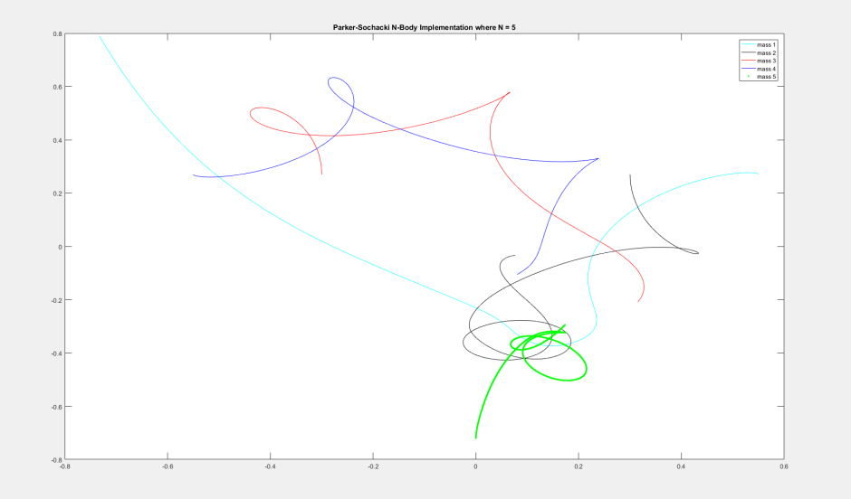
This is simply chaotic motion with 5 bodies
number of bodies = 5
G = 1
mass of particle 1 = 1
mass of particle 2 = 1
mass of particle 3 = 1
mass of particle 4 = 1
mass of particle 5 = 1
Order of Maclaurin series = 7
time step = 0.005
number of frames = 180
x_particle 1 = 0.55
velocity_x_particle 1 = 0
y_particle 1 = 0.27
velocity_y_particle 1 = 0.23
x_particle 2 = 0.3
velocity_x_particle 2 = 0
y_particle 2 = 0.27
velocity_y_particle 2 = -2.42
x_particle 3 = -0.30
velocity_x_particle 3 = 0
y_particle 3 = 0.27
velocity_y_particle 3 = 2.42
x_particle 4 = -0.55
velocity_x_particle 4 = 0
y_particle 4 = 0.27
velocity_y_particle 4 = -0.23
x_particle 5 = 0
velocity_x_particle 5 = 0
y_particle 5 = -0.72
velocity_y_particle 5 = 0
These are all of the examples I tried but you can play with the code to any number of particles you would like to get some interesting patterns!
I have a final note on the order and time step. If you look, some simulations had much smaller time steps than others. My smallest time step was 0.001 while my largest time step was 0.01. My lowest order was 7 while my highest order was 30. I was solving the same system of Ordinary Differential Equations. The only differences were in the initial conditions. If I were using other numerical methods like Euler, Verlet, Leap Frog, or Runge Kutta, I could only adjust the time step(I would have to rewrite Runge-Kutta to get methods like Runge-Kutta 2nd Order, Runge-Kutta 3rd Order, and Runge-Kutta 4th Order). If my order was too low with Parker-Sochacki, I only had to change that value and run the simulation again. With the Parker-Sochacki method, I was able to play with both time step and order just by changing what those values are set to.
I also came across the same “close encounters” benefit in the 5-body problem. If I lowered the order too much, the particles would all diverge. I could compensate by lowering the time step or raising the order of the Maclaurin series. I did this experimentally.
Take care and have a happy 4th of July!
Sincerely,
Adam Wermus
